Introduction to rPHG2

The basic workflow of the rPHG2 package is as follows:

Create a connection object
Read data into the R environment
Analyze and visualize data retrieval

This document introduces you to rPHG2’s methods and grammar, and shows you how to apply them to the previously mentioned workflow.

Creating connection objects

rPHG objects can be created through two primary sources: * local data * server connections

Creating initial “connection” objects helps unify downstream reading and evaluation steps for PHGv2 data. In the next couple of sections, we will show you how to create either local or server connnection objects.

Local data

Local connections are for local TileDB instances or direct locations of hVCF files on a local disk. To create a local connection, we will create a PHGLocalCon object using the following constructor function:

PHGLocalCon()

For the above example, we will create a connection to some example local hVCF files provided with the rPHG2 package:

LineA.h.vcf
LineB.h.vcf

Since the full paths to these files will differ between each user, we can use the system.file() function to get the full path:

system.file("extdata", "LineA.h.vcf", package = "rPHG2")

This will get the full path from the extdata directory for the file, LineA.h.vcf, found in the rPHG2 source code.

We can further build on this to create a collection of full file paths to our hVCF data:

hVcfFiles <- system.file(
    "extdata", 
    c("LineA.h.vcf", "LineB.h.vcf"), 
    package = "rPHG2"
)

Now that we have a collection of hVCF files, we can use the PHGLocalCon() constructor function to create a PHGLocalCon object:

localCon <- hVcfFiles |> PHGLocalCon()

localCon

## A PHGLocalCon connection object
##  ❯ DB URI.......: ◻
##  ❯ hVCF Files...: ◼

Additionally, if you have a directory of valid hVCF files, you can simply pass the directory path to the constructor. In the following example, I will point to the extdata data directory without pointing to singular hVCF files that is found within the package:

system.file("extdata", package = "rPHG2") |> PHGLocalCon()

## A PHGLocalCon connection object
##  ❯ DB URI.......: ◻
##  ❯ hVCF Files...: ◼

From here, we can move to the next section to create a HaplotypeGraph object interface with the JVM.

Server connections

Note

We are still actively working on this section and will not have the same compatibility as rPHG. Stay tuned for further details!

Conversely, server locations are for databases served on publicly available web services leveraging the Breeding API (BrAPI) endpoints. Since this is a connection to a server, a URL path instead of a local file path will be needed. We will use the PHGServerCon() constructor function to create a PHGServerCon object:

srvCon <- "phg.maizegdb.org" |> PHGServerCon()

srvCon

## A PHGServerCon connection object
##  ❯ Host............: phg.maizegdb.org
##  ❯ Server Status...: 200 (OK)

In the above example, we have made the assumptions that this URL:

Uses a secure transfer protocol (https)
Uses default ports for data serving
Has BrAPI specified endpoints

For points 1 and 2, if the URL uses non-secure protocols (“http”) and/or has a modified port number, you will need to specify these with the protocol and port parameters in the constructor function. For example:

"www.my-unsecure-phg.org" |> 
    PHGServerCon(
        port     = 5300, 
        protocol = "http"
    )

For point 3, if the constructor cannot resolve mandatory endpoints, an exception will occur.

Creating JVM objects

Note

This will require the rJava package to be installed along with a modern version of Java (e.g., $\geq$ v17) to work properly!

Now that we have either a local or server-based connection object, we can convert the raw hVCF data into a HaplotypeGraph JVM object and bridge the Java reference pointer to R. Before we build the JVM graph object, we need to initialize the JVM and add the JAR files to our environment that are found within the latest distribution of PHGv2.

Note: If you have not downloaded this, please see instructions here before you continue!

To initialize, run the following command:

initPhg("phg/path/to/lib")

…where phg/path/to/lib is the lib directory found within the decompressed release of PHGv2. Now that the JVM has been initialized, we can build the JVM graph using buildHaplotypeGraph() using the local connection object as input:

graph <- localCon |> buildHaplotypeGraph()

graph

## A HaplotypeGraph object @ 2e32ccc5
##  ❯ # of ref ranges....: 38
##  ❯ # of samples.......: 2
##  ❯ # of chromosomes...: 2

In the above example, we took the local connection object and passed it into a HaplotypeGraph constructor. Here, we have a basic class that contains a pointer object where we can direct data from Java to R:

graph |> javaRefObj()

## [1] "Java-Object{net.maizegenetics.phgv2.api.HaplotypeGraph@2e32ccc5}"

Returning version and memory values

Since we need to construct an interface to a local instance of Java, errors may arise due to several issues. Two common causes are version issues and memory allocated to the JVM. For debugging and monitoring purposes, we can use the jvmStats() function which creates a instance of a JvmStats object.

javaStats <- jvmStats()

javaStats

## General Stats:
##  ❯ # of JARs......: 228
##  ❯ Java version...: 17.0.13
##  ❯ PHG version....: 2.4.39.194
## 
## Memory Stats (GB):
##  ❯ Max............: 0.5
##  ❯ Total..........: 0.246
##  ❯ Free...........: 0.223
##  ❯ Allocated......: 0.023

This object contains several values:

Total number of PHGv2 JAR files added to the class path
Your local Java version
The current PHGv2 version added to the class path
Current memory allocation to the JVM (recorded in gigabytes [GB])

Reading data

Now that we have created a HaplotypeGraph object, we can begin reading data using the read* family of rPHG2 functions.

Sample IDs

To return a vector of sample IDs from the graph object, we can use the readSamples() function:

graph |> readSamples()

## [1] "LineA" "LineB"

Reference ranges

To return information about all reference ranges found within the graph object, we can use the readRefRanges() function. This will return a GRanges object which is a common data class in the GenomicRanges package:

graph |> readRefRanges()

## GRanges object with 38 ranges and 1 metadata column:
##        seqnames      ranges strand |         rr_id
##           <Rle>   <IRanges>  <Rle> |   <character>
##    [1]        1      1-1000      * |      1:1-1000
##    [2]        1   1001-5500      * |   1:1001-5500
##    [3]        1   5501-6500      * |   1:5501-6500
##    [4]        1  6501-11000      * |  1:6501-11000
##    [5]        1 11001-12000      * | 1:11001-12000
##    ...      ...         ...    ... .           ...
##   [34]        2 38501-39500      * | 2:38501-39500
##   [35]        2 39501-44000      * | 2:39501-44000
##   [36]        2 44001-45000      * | 2:44001-45000
##   [37]        2 45001-49500      * | 2:45001-49500
##   [38]        2 49501-50500      * | 2:49501-50500
##   -------
##   seqinfo: 2 sequences from an unspecified genome; no seqlengths

Haplotype IDs

To return all haplotype IDs as a “sample $\times$ reference range” matrix object, we can use the readHapIds() function:

m <- graph |> readHapIds()

# Show only first 3 columns
m[, 1:3]

##          1:1-1000                           1:1001-5500                       
## LineA_G1 "12f0cec9102e84a161866e37072443b7" "3149b3144f93134eb29661bade697fc6"
## LineB_G1 "4fc7b8af32ddd74e07cb49d147ef1938" "8967fabf10e55d881caa6fe192e7d4ca"
##          1:5501-6500                       
## LineA_G1 "1b568197f6f329ec5b71f66e49a732fb"
## LineB_G1 "05efe15d97db33185b64821791b01b0f"

Haplotype ID metadata

To return metadata for each haplotype ID as a tibble object, we can use the readHapIdMetaData() function:

graph |> readHapIdMetaData()

## # A tibble: 76 × 6
##    hap_id                 sample_name description source checksum ref_range_hash
##    <chr>                  <chr>       <chr>       <chr>  <chr>    <chr>         
##  1 0eb9029f3896313aebc69… LineA       haplotype … /User… Md5      39f96726321b3…
##  2 12f0cec9102e84a161866… LineA       haplotype … /User… Md5      546d1839623a5…
##  3 13417ecbb38b9a159e3ca… LineA       haplotype … /User… Md5      5812acb1aff74…
##  4 18498579d89483ac270e8… LineA       haplotype … /User… Md5      e07d04d2fc96b…
##  5 184a72815a2ba5949635c… LineA       haplotype … /User… Md5      cb86faf105b19…
##  6 1b568197f6f329ec5b71f… LineA       haplotype … /User… Md5      d896e9cc56e74…
##  7 1e38bd82670c3f10982f7… LineA       haplotype … /User… Md5      db22dfc14799b…
##  8 3149b3144f93134eb2966… LineA       haplotype … /User… Md5      57705b1e2541c…
##  9 369464a8743d2e40ad83d… LineA       haplotype … /User… Md5      66465399052d8…
## 10 3ec680649615da0685b8c… LineA       haplotype … /User… Md5      347f0478b1a55…
## # ℹ 66 more rows

Haplotype ID metadata (positions)

To return positional information for each haplotype ID as another tibble object, we can use the readHapIdPosMetaData() function:

graph |> readHapIdPosMetaData()

## # A tibble: 76 × 5
##    hap_id                           contig_start contig_end start   end
##    <chr>                            <chr>        <chr>      <int> <int>
##  1 0eb9029f3896313aebc69c8489923141 2            2          49501 50300
##  2 12f0cec9102e84a161866e37072443b7 1            1              1  1000
##  3 13417ecbb38b9a159e3ca8c9dade7088 2            2              1  1000
##  4 18498579d89483ac270e8cca57f34752 1            1          16501 17500
##  5 184a72815a2ba5949635cc38769cedd0 2            2          12001 16500
##  6 1b568197f6f329ec5b71f66e49a732fb 1            1           5501  6500
##  7 1e38bd82670c3f10982f70390c599a8d 2            2          16501 17500
##  8 3149b3144f93134eb29661bade697fc6 1            1           1001  5500
##  9 369464a8743d2e40ad83d1375c196bdd 1            1           6501 11000
## 10 3ec680649615da0685b8c245e0f196e2 2            2          11001 12000
## # ℹ 66 more rows

All hVCF data

In a majority of cases, we may need more than one piece of hVCF data. We can read all of the prior data simultaneously as PHGDataSet object which is an in-R-memory representation of all hVCF data:

phgDs <- graph |> readPhgDataSet()
phgDs

## A PHGDataSet object
##  ❯ # of ref ranges....: 38
##  ❯ # of samples.......: 2
## ---
##  ❯ # of hap IDs.......: 76
##  ❯ # of asm regions...: 76

If this object is created, we can use the prior read* methods to instantaneously pull out the previously mentioned R data objects:

Filter data

In some cases, you may want to query information and focus on one specific reference range and/or sample(s). We can filter our PHGDataSet objects using the filter* family of functions.

For the following examples, let’s picture our primary data as a 2-dimensional matrix of:

samples (rows)
reference ranges (columns)
hap ID data (elements)

If we were to represent this as an object in R called phgDs, it would look like the following diagram:

phgDs

## A PHGDataSet object
##  ❯ # of ref ranges....: 38
##  ❯ # of samples.......: 2
## ---
##  ❯ # of hap IDs.......: 76
##  ❯ # of asm regions...: 76

…where each individual colored cell is a haplotype ID.

Filter by sample

If we want to filter based on sample ID, we can use the filterSamples() function. Simply add the sample ID or collection of sample IDs as a character string or a vector of character strings, respectively. Using the prior diagram as a reference, I will filter out anything that is not the following:

B73
Ky21
Mo17

phgDs |> filterSamples(c("B73", "Ky21", "Mo17"))

Note: If samples are added to the filter collection, but are not present in the data, they will be discarded. If no samples are found, an exception will be thrown stating that no samples could be found.

Filter by reference range

If we want to filter based on sample ID, we can use the filterRefRanges() function. Currently, this takes a GRanges object where we can specify integer-based ranges located in genomic regions by chromosome (i.e., seqnames). For example, if I want to return all ranges that intersect with the following genomic regions:

Chromosome	Start (bp)	End (bp)
`"1"`	`100`	`400`
`"2"`	`400`	`900`

I can create the following GRanges object and pass that to the filter method:

gr <- GRanges(
    seqnames = c("1", "2"),
    ranges = IRanges(
        c(100, 800),
        c(400, 900)
    )
)


phgDs |> filterRefRanges(gr)

Chaining methods

Since we have two dimensions, we can filter simultaneously by “piping” or combining filter methods in one pass:

gr <- GRanges(
    seqnames = c("1", "2"),
    ranges = IRanges(
        c(100, 800),
        c(400, 900)
    )
)

phgDs |> 
    filterSamples(c("B73", "Ky21", "Mo17")) |> 
    filterRefRanges(gr)

Summarize and visualize data

In addition to parsing multiple hVCF files into R data objects via a PHGDataSet, rPHG2 also provides functions to summarize and visualize data.

Global values

To begin, we can return general values on the number of observations within our dataset using the numberOf* family of functions:

phgDs

## A PHGDataSet object
##  ❯ # of ref ranges....: 38
##  ❯ # of samples.......: 2
## ---
##  ❯ # of hap IDs.......: 76
##  ❯ # of asm regions...: 76

# Get number of samples/taxa
phgDs |> numberOfSamples()

## [1] 2

# Get number of chromosomes
phgDs |> numberOfChromosomes()

## [1] 2

# Get number of reference ranges
phgDs |> numberOfRefRanges()

## [1] 38

# Get number of haplotype IDs
phgDs |> numberOfHaplotypes()

## [1] 76

Get counts of unique haplotype IDs

To get the unique number of haplotypes per reference range in our PHGDataSet object, we can use numberOfHaplotypes() again, but set the internal parameter byRefRange to TRUE:

phgDs |> numberOfHaplotypes(byRefRange = TRUE)

## # A tibble: 38 × 7
##    rr_id         n_haplo seqnames start   end width strand
##    <chr>           <int> <fct>    <int> <int> <int> <fct> 
##  1 1:1-1000            2 1            1  1000  1000 *     
##  2 1:1001-5500         2 1         1001  5500  4500 *     
##  3 1:11001-12000       2 1        11001 12000  1000 *     
##  4 1:12001-16500       2 1        12001 16500  4500 *     
##  5 1:16501-17500       2 1        16501 17500  1000 *     
##  6 1:17501-22000       2 1        17501 22000  4500 *     
##  7 1:22001-23000       2 1        22001 23000  1000 *     
##  8 1:23001-27500       2 1        23001 27500  4500 *     
##  9 1:27501-28500       2 1        27501 28500  1000 *     
## 10 1:28501-33000       2 1        28501 33000  4500 *     
## # ℹ 28 more rows

Visualize counts of unique haplotype IDs

We can visualize the prior section using a member of the plot* family of functions, plotHaploCounts(). By default, this will produce a scatter plot of data found across all reference ranges in the reference genome (similar to a Manhattan plot):

phgDs |> plotHaploCounts()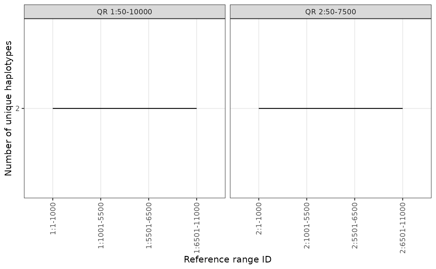

To get more “granular” views of specific regions within our data, we can pass a GRanges object from the package GenomicRanges to the gr parameter:

# library(GenomicRanges)

query <- GRanges(
    seqnames = "1", 
    ranges = IRanges(start = 50, end = 10000)
)

phgDs |> plotHaploCounts(gr = query)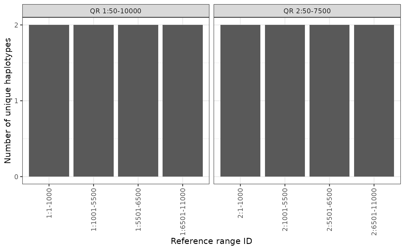

We can also query mutltiple regions of interest simultaneously by adding more observations to the query object:

# library(GenomicRanges)

query <- GRanges(
    seqnames = c("1", "2"), 
    ranges = IRanges(start = c(50, 50), end = c(10000, 7500))
)

phgDs |> plotHaploCounts(gr = query)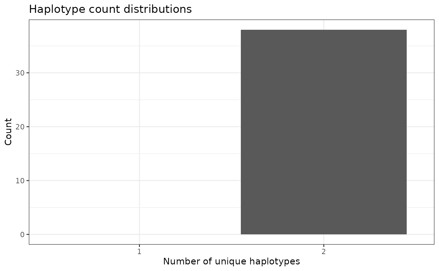

Finally, we provide 3 separate “geometry” options for plotting using the geom parameter: * "l" - line plotting (e.g., geom_line()) (default) * "b" - bar plotting (e.g., geom_bar()) * "p" - point plotting (e.g., geom_point())

For example, if we want to switch this from a line plot to a bar plot, we can specify geom = "b":

phgDs |> plotHaploCounts(gr = query, geom = "b")

Visualize distributions of unique haplotype IDs

To get a more “global” estimate of unique haplotype ID distribution across the genome, we can us the function plotHaploDist():

phgDs |> plotHaploDist()

Returning sequence data

We can also return haplotype sequence information via the readSequence() command with PHG data sets (i.e., PHGDataSet objects) pointed to PHGv2 databases containing compressed assemblies information.

In order to perform sequence retrieval, we must perform a couple of steps:

Add host information to a PHGLocalCon object
Add an AGC path to the global options (i.e., the options() function)

Setup - add host information

For step 1, during the the construction of a PHGLocalCon object using the PHGLocalCon() function, add the path to a PHGv2 database containing a compressed sequence file:

dbPath <- "/my/phgv2/db_path/"

# using 'hVcfFiles' variable from earlier steps
localCon <- hVcfFiles |> PHGLocalCon(dbUri = dbPath)

If you are unsure what this path is, it should be the directory that was created during the PHGv2 building and loading steps and contains files and sub-directories that looks like the following:

phg_v2_example/
├── data
│   ├── anchors.gff
│   ├── annotation_keyfile.txt
│   ├── Ref-v5.fa
│   ├── LineA-final-01.fa
│   └── LineB-final-04.fa
├── output
│   └── updated_assemblies
│       ├── Ref.fa
│       ├── LineA.fa
│       └── LineB.fa
└── vcf_dbs
    ├── assemblies.agc *
    ├── gvcf_dataset/
    ├── hvcf_dataset/
    └── temp/

Note

In order for this to work, this directory/database must contain a compressed sequence file. By default, this file will be called assemblies.agc. This is a compressed file generated by the Assembled Genomes Compressor.

Setup - add AGC path

For step 2, we must also have a working AGC application for our operating system and environment. This can be established in a couple of ways:

Option 1 - Conda

If you went through the steps of setting up a PHG database on your working machine, we can assume that you have:

A working Conda installation
A working PHGv2 Conda environment. This by default will be called phgv2-conda.

If this is the case, you will, by default, have AGC already set up on your machine since this is a necessary application for several crucial PHGv2 steps. You can verify AGC is present in your PHGv2 environment by running the following command within a terminal:

conda run -n phgv2-conda agc

If present, this will output a series of commands used by the agc program. For example:

$ conda run -n phgv2-conda agc

AGC (Assembled Genomes Compressor) v. 3.1.0 [build 20240312.1]
Usage: agc <command> [options]
Command:
   create   - create archive from FASTA files
   append   - add FASTA files to existing archive
   getcol   - extract all samples from archive
   getset   - extract sample from archive
   getctg   - extract contig from archive
   listref  - list reference sample name in archive
   listset  - list sample names in archive
   listctg  - list sample and contig names in archive
   info     - show some statistics of the compressed data
Note: run agc <command> to see command-specific options

Note

If you have changed the name of your environment, the value given with the -n flag will have to change!

If your machine matches the prior criteria, you may use the rPHG2 function linkCondaBin() to link your Conda environment’s AGC application path to R’s global options:

linkCondaBin(condaPath = "/path/to/my/conda/installation")

This function will assume your environment name is called phgv2-conda. If you have a different, you can add the modified id to the envName parameter.

linkCondaBin(
    condaPath = "/path/to/my/conda/installation",
    envName   = "phgv2-sorghum" # example Conda environment name
)

Option 2 - manual AGC path

If you do not have Conda installed or no PHGv2 instance, but have AGC installed on your machine, you can manually set the path using R’s option() function. In order for rPHG2 to correctly identify the correct path, you must make a new key in the global options called phgv2_agc_path:

options("phgv2_agc_path" = "/path/to/my/agc/application/bin/agc")

Note

This must be the path to the AGC binary (i.e., the file named agc) found in the release.

Setup - build `PHGDataset` object

Now that all prerequisites are completed, we can finish building the PHGDataSet object using conventional rPHG2 syntax:

phgDs <- localCon
    buildHaplotypeGraph() |>
    readPhgDataSet()

phgDs

## A PHGDataSet object
##  ❯ # of ref ranges....: 38
##  ❯ # of samples.......: 2
## ---
##  ❯ # of hap IDs.......: 76
##  ❯ # of asm regions...: 76

Using `readSequence()`

Now that we have our PHGDataSet object created, we can return specific sequence information relating to an individual haplotype or a collection of haplotypes using a haplotype or reference range identifier, respectively. Similar to other syntax, we can simply pipe our PHGDataSet object into the readSequence() method.

For starters, I will return a single haplotype sequence using the hapId parameter:

# Return first haplotype ID in matrix (example)
hapId <- phgDs |> readHapIds() |> _[1, 1]

phgDs |> readSequence(hapId = hapId)

## DNAStringSet object of length 1:
##     width seq                                               names               
## [1]  1000 GCGCGGGGACCGAGAAACCCGGC...CCACGCACAGGCGAGGGAACGGC 1 sampleName=Line...

The data object that is returned from readsequence() is a dnastringset object which is from the Biostrings package found on bioconductor. you can think of this object a list of dnastringset objects which are memory-efficient representations of biological sequences (e.g., dna). this will allow users the ability to access all Biostrings-related methods for objects of type dnastring. For more information about how to use these objects, take a look at the “Quick Overview” documentation found in the Biostrings package.

If we are interested in returning haplotype sequence data from an entire reference range, we can specify a reference range ID using the rrId parameter. This identifier will be a character object containing the following pattern:

<chromosome_id>:<start_bp>-<end_bp>

For example, this identifier will look like the following “first” reference range found in our example hVCF data:

# Return first reference range in matrix (example)
rrId <- phgDs |> readHapIds() |> colnames() |> _[1]

rrId

## [1] "1:1-1000"

phgDs |> readSequence(rrId = rrId)

## DNAStringSet object of length 2:
##     width seq                                               names               
## [1]  1000 GCGCGGGGACCGAGAAACCCGGC...CCACGCACAGGCGAGGGAACGGC 1 sampleName=Line...
## [2]  1000 GCGCGGGGACCGTGAAACCCGGC...CCACGCACAGGCGAGGTAACGGC 1 sampleName=Line...