Load and visualize PHG metrics

Creating `PHGMetrics` objects

In addition to loading and inspecting hVCF data, rPHG2 provides classes for quick loading and granular visualization of “PHG metrics” data. Currently, there are two primary types of PHG metrics:

Alignment files from AnchorWave
- used for collinearity plotting of samples against the reference genome
gVCF data metrics
- general statistics of gVCFs generated for each sample $\times$ chromosome pair

To provide “easy to use” downstream plotting methods, we will need to construct a new rPHG2 PHGMetrics object by providing either file paths, directory paths, or a combination of the two as a character vector. In the following example, I will provide a path to a directory containing both alignment and gVCF data that is found within the library:

metricDir <- system.file("extdata", package = "rPHG2")

metricDir

## [1] "/home/runner/work/_temp/Library/rPHG2/extdata"

From this variable, we can simply pass this to the PHGMetrics constructor, PHGMetrics():

metData <- PHGMetrics(metricDir)

##  ✔ reading data for: toy_gvcf_metrics.tsv
##  ✔ reading data for: toy_anchors_s01.anchorspro

metData

## A PHGMetrics object containing 2 tables:
## -- AnchorWave data:
##  ❯ toy_anchors_s01 (969 10)
## -- gVCF data:
##  ❯ toy_gvcf_metrics (41 19)

Accessing metrics data tables

General use

From the previously created metData object, we can directly access various types of data through a series of accessor methods.

If we want to extract all metrics tables as data.frame-like objects, we can use the metricsTable() function, which will return a list object of data.frame tables:

metData |> metricsTable()

## $toy_anchors_s01
## # A tibble: 969 × 10
##    ref_chr reference_start reference_end query_chr query_start query_end strand
##      <int>           <int>         <int>     <int>       <int>     <int> <chr> 
##  1       1           52892         53561         1       22637     23277 +     
##  2       1          275401        278445         1      196230    199275 +     
##  3       1          665653        669559         1      456629    460535 +     
##  4       1          723978        724529         1      514619    515170 +     
##  5       1         1031998       1033805         1      788012    789822 +     
##  6       1         1497930       1503054         1     1250572   1255668 +     
##  7       1         1517777       1519239         1     1270343   1271805 +     
##  8       1         2466395       2468560         1     2047907   2050072 +     
##  9       1         2533102       2536854         1     2093924   2097674 +     
## 10       1         2638837       2639286         1     2188800   2189249 +     
## # ℹ 959 more rows
## # ℹ 3 more variables: gene <chr>, block_index <int>, score <dbl>
## 
## $toy_gvcf_metrics
## # A tibble: 41 × 19
##    taxa  chrom ref_length num_snps num_ins num_del  num_ns num_bases_inserted
##    <chr> <chr>      <int>    <int>   <int>   <int>   <int>              <int>
##  1 Xb01  ALL    473519425  2706357  336754  301867 2101168           41462213
##  2 Xb01  Vu01    42129361   154059   26280   20211  181091            2600647
##  3 Xb01  Vu02    33908088   178101   21457   18981  152494            2293028
##  4 Xb01  Vu03    65292630   273800   43347   38073  284407            2694624
##  5 Xb01  Vu04    42731077   424488   34561   31514  177567            3908337
##  6 Xb01  Vu05    48746289   183067   28355   24918  224956            4352143
##  7 Xb01  Vu06    34463471   149413   22663   20431  152644            2262451
##  8 Xb01  Vu07    40876636   164945   26583   23708  178058            1966857
##  9 Xb01  Vu08    38363498   191440   26010   24047  171568            2214889
## 10 Xb01  Vu09    43933251   191892   27914   23807  187467            3967889
## # ℹ 31 more rows
## # ℹ 11 more variables: num_bases_deleted <int>,
## #   percent_identity_with_ref <dbl>, percent_mapped_to_ref <dbl>,
## #   mean_insertion_size <dbl>, median_insertion_size <dbl>,
## #   largest_insertion <int>, mean_deletion_size <dbl>,
## #   median_deletion_size <dbl>, largest_deletion <int>,
## #   ref_ranges_with_haplotype <int>, haplotypes_identical_to_ref <int>

Individual table selection

If we want to extract just one table, we can provide the name of the table into the metricsTable() function by specifying a valid name with the name parameter. By default, the PHGMetrics() constructor will specify the names of each table by extracting the base name of each file passed to the constructor. For example, if we have the following file path:

/path/to/my/alignment_file.anchorspro

…the default name for this table will be alignment_file. Depending on the complexity of the file ID, rPHG2 provides a $ operator override which allows users to cycle through valid metrics table names:

metData |> metricsTable(name = metData$toy_anchors_s01)

## # A tibble: 969 × 10
##    ref_chr reference_start reference_end query_chr query_start query_end strand
##      <int>           <int>         <int>     <int>       <int>     <int> <chr> 
##  1       1           52892         53561         1       22637     23277 +     
##  2       1          275401        278445         1      196230    199275 +     
##  3       1          665653        669559         1      456629    460535 +     
##  4       1          723978        724529         1      514619    515170 +     
##  5       1         1031998       1033805         1      788012    789822 +     
##  6       1         1497930       1503054         1     1250572   1255668 +     
##  7       1         1517777       1519239         1     1270343   1271805 +     
##  8       1         2466395       2468560         1     2047907   2050072 +     
##  9       1         2533102       2536854         1     2093924   2097674 +     
## 10       1         2638837       2639286         1     2188800   2189249 +     
## # ℹ 959 more rows
## # ℹ 3 more variables: gene <chr>, block_index <int>, score <dbl>

Table selection by metric type

We can also extract tables by type using the type parameter in the metricsTable() function. Currently, the two metric types that PHGv2 provides are as follows:

align - For AnchorWave alignment files
gvcf - For gVCF metrics files

metData |> metricsTable(type = "gvcf")

## # A tibble: 41 × 19
##    taxa  chrom ref_length num_snps num_ins num_del  num_ns num_bases_inserted
##    <chr> <chr>      <int>    <int>   <int>   <int>   <int>              <int>
##  1 Xb01  ALL    473519425  2706357  336754  301867 2101168           41462213
##  2 Xb01  Vu01    42129361   154059   26280   20211  181091            2600647
##  3 Xb01  Vu02    33908088   178101   21457   18981  152494            2293028
##  4 Xb01  Vu03    65292630   273800   43347   38073  284407            2694624
##  5 Xb01  Vu04    42731077   424488   34561   31514  177567            3908337
##  6 Xb01  Vu05    48746289   183067   28355   24918  224956            4352143
##  7 Xb01  Vu06    34463471   149413   22663   20431  152644            2262451
##  8 Xb01  Vu07    40876636   164945   26583   23708  178058            1966857
##  9 Xb01  Vu08    38363498   191440   26010   24047  171568            2214889
## 10 Xb01  Vu09    43933251   191892   27914   23807  187467            3967889
## # ℹ 31 more rows
## # ℹ 11 more variables: num_bases_deleted <int>,
## #   percent_identity_with_ref <dbl>, percent_mapped_to_ref <dbl>,
## #   mean_insertion_size <dbl>, median_insertion_size <dbl>,
## #   largest_insertion <int>, mean_deletion_size <dbl>,
## #   median_deletion_size <dbl>, largest_deletion <int>,
## #   ref_ranges_with_haplotype <int>, haplotypes_identical_to_ref <int>

Other accessor functions

In addition to extracting tables, we can also access other types of data found in PHGMetrics objects.

Identifiers

If we want to return all IDs of every table we can use the metricsIds() function:

metData |> metricsIds()

## [1] "toy_anchors_s01"  "toy_gvcf_metrics"

Similar to the previous section, we can also return IDs by metric type using the type parameter:

metData |> metricsIds(type = "align")

## [1] "toy_anchors_s01"

Metadata

We can also extract metadata which will provide a simple data.frame table containing three columns:

file - file ID of loaded data
type - metrics data type
id - the “name” of the metrics table

metData |> metricsMetaData()

## # A tibble: 2 × 3
##   file                       type  id              
##   <chr>                      <chr> <chr>           
## 1 toy_gvcf_metrics.tsv       gvcf  toy_gvcf_metrics
## 2 toy_anchors_s01.anchorspro align toy_anchors_s01

Updating `PHGMetrics` objects

To update existing PHGMetrics we can use f()<- complements to the accessor methods from the prior sections. Currently, we can update or add the following information:

metrics table names/IDs (update)
metrics tables (add)

Update metric IDs

To update pre-existing names of tables in the object, we can use the metricsIds() function in conjunction with the assignment (<-) operator by passing a named character vector, where the name of the vector is the name of the old table ID and the element is the new name:

nameMap <- c(
    "old_id1" = "new_id1",
    "old_id2" = "new_id2"
)

If we do not wish to remember all old IDs of our tables, we can use the prior $ operator in conjunction with rPHG2’s defined “to” operator, %T% in a vector:

nameMap <- c(
    metData$toy_gvcf_metrics %T% "new_gvcf_id",
    metData$toy_anchors_s01 %T% "new_anchor_id"
)

The prior code will internally evaluate to named character vector:

nameMap

## toy_gvcf_metrics  toy_anchors_s01 
##    "new_gvcf_id"  "new_anchor_id"

This can be passed to the metricsIds() function:

metricsIds(metData) <- nameMap

metData |> metricsIds()

## [1] "new_anchor_id" "new_gvcf_id"

Update chromosome IDs

To update pre-existing chromosome IDs found within a PHGMetrics object, we can use the seqnames() in conjunction with the assignment (<-) operator by passing a data.frame object that contains two columns:

old_id - old chromosome IDs already present in the object
new_id - the new name for the ID

We can also use this function to return all global chromosome IDs from the object:

# Make copy for example purposes
metNew <- metData

metNew |> seqnames()

##  [1] "1"          "2"          "3"          "Vu01"       "Vu02"      
##  [6] "Vu03"       "Vu04"       "Vu05"       "Vu06"       "Vu07"      
## [11] "Vu08"       "Vu09"       "Vu10"       "Vu11"       "contig_206"
## [16] "contig_178"

To update, simply pass the data.frame object with the old and new ID maps to the seqnames() function:

keyFile <- data.frame(
    old_id = c("Vu01", "Vu03"),
    new_id = c("CHR_01", "CHR_03")
)

seqnames(metNew) <- keyFile

metNew |> seqnames()

##  [1] "1"          "2"          "3"          "CHR_01"     "Vu02"      
##  [6] "CHR_03"     "Vu04"       "Vu05"       "Vu06"       "Vu07"      
## [11] "Vu08"       "Vu09"       "Vu10"       "Vu11"       "contig_206"
## [16] "contig_178"

As you can see, all instances of "Vu01" and "Vu03" have been globally changed to "CHR_01" and "CHR_03".

Update tables

We can also add new tables to our existing PHGMetrics objects using the metricsTable() function by passing a named list object containing a combination of the valid types:

file paths
directory paths
in-memory R data.frame objects containing valid PHGv2 metric structures

For this example, I will add another table via a data.frame using some internal toy data found in the rPHG2 package:

algnPath <- system.file("extdata/toy_anchors_s01.anchorspro", package = "rPHG2")
algnDf   <- read.table(algnPath, header = TRUE, sep = "\t")

head(algnDf)

##   refChr referenceStart referenceEnd queryChr queryStart queryEnd strand
## 1      1          52892        53561        1      22637    23277      +
## 2      1         275401       278445        1     196230   199275      +
## 3      1         665653       669559        1     456629   460535      +
## 4      1         723978       724529        1     514619   515170      +
## 5      1        1031998      1033805        1     788012   789822      +
## 6      1        1497930      1503054        1    1250572  1255668      +
##          gene blockIndex   score
## 1    OQU90574         40 0.83871
## 2 interanchor         40      NA
## 3    KXG37092         40 1.00000
## 4    KXG37098         40 1.00000
## 5    EER93094         40 1.00000
## 6    KXG37167         40 1.00000

metricsTable(metData) <- list("new_algn_table" = algnDf)

##  ✔ importing data for: new_algn_table

metData |> metricsMetaData()

## # A tibble: 3 × 3
##   file                       type  id            
##   <chr>                      <chr> <chr>         
## 1 toy_gvcf_metrics.tsv       gvcf  new_gvcf_id   
## 2 toy_anchors_s01.anchorspro align new_anchor_id 
## 3 new_algn_table             align new_algn_table

Visualize metrics data

If you are satisfied with how the metrics data is loaded into R, we can directly visualize granular diagnostic plots using the plot* family of functions.

AnchorWave data

For example, if I want to generate dot plots from alignment data, I can simply pass the PHGMetrics object to the function, plotDot(). Currently this can only plot one table at a time, so we must specify the alignment table that we want to visualize:

metData |> plotDot(metData$new_anchor_id)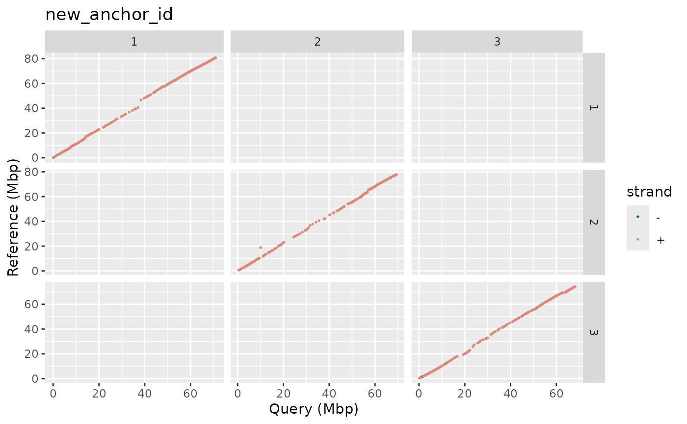

Note: This plot can only work on alignment (type = "align") data and will throw an error if any gVCF-based metrics Ids are used.

If only one AnchorWave table is loaded into memory, a user can also specify a more simpler approach:

metData |> plotDot()

Note: If more than one table is loaded, this approach will still work, but will pick the first table/elemement in the internal list object.

gVCF metrics data

We can also visualize gVCF data using the function plotGvcf(). This method provides granular means of visualizing various forms of metrics data found within the gVCF metrics file.

This method takes 3 primary components:

The PHGMetrics object
A metric ID
A gVCF metric ID $\sim$ contig ID formula

A simple approach would be to pass the PHGMetrics object along with the specified metrics ID:

metData |> plotGvcf(metData$new_gvcf_id)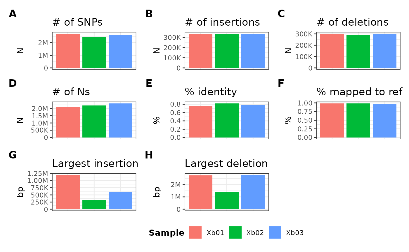

Similar to the alignment approach, if you have just one table, you can also pass just the function, since it will dynamically pick the only table:

metData |> plotGvcf()

Formula usage

For more “granular” approaches, we can specify a formula (f) to dictate what types of metrics and chromosome IDs we want plotted using the following logic:

<gvcf metric ids> ~ <contig ids>

The following are valid metric IDs:

Metric ID	Description
`ref_length`	The length of the reference sequence
`num_snps`	The number of SNP records in the gVCF file for the given chromosome
`num_ins`	The number of insertion records in the gVCF file
`num_del`	The number of deletion records in the gVCF file
`num_ns`	The number of N’s/ambiguous bases in the assembly alignment
`num_bases_inserted`	The number of bases inserted relative to the reference sequence
`num_bases_deleted`	The number of bases deleted relative to the reference sequence
`percent_identity_with_ref`	The proportion of bases relative to refLength that are the same base as the reference base
`percent_mapped_to_ref`	The proportion of bases relative to refLength that are present in a gVCF record
`mean_insertion_size`	The mean size of insertion records
`median_insertion_size`	The median size of insertion records
`largest_insertion`	The size of the largest insertion
`mean_deletion_size`	The mean size of deletion records
`median_deletion_size`	The median size of deletion records
`largest_deletion`	The size of the largest deletion

Due to the number of metric IDs, several “collection” IDs are also valid:

Collection ID	Description
`ALL`	Plots all prior metric IDs
`CORE`	Plots `num_snps`, `num_ins`, `num_del`, `num_ns`, `percent_identity_with_ref`, `percent_mapped_to_ref`, `largest_insertion`, `largest_deletion`

Note: Collection IDs may only be plotted one at a time or else an error will be thrown.

For example, if I want to plot:

the length of the reference sequence (ref_length)
the number of deletions (num_del)

…for chromsomes:

Vu01
Vu05

…I can use the following formula syntax:

metData |> plotGvcf(f = ref_length + num_del ~ Vu01 + Vu05)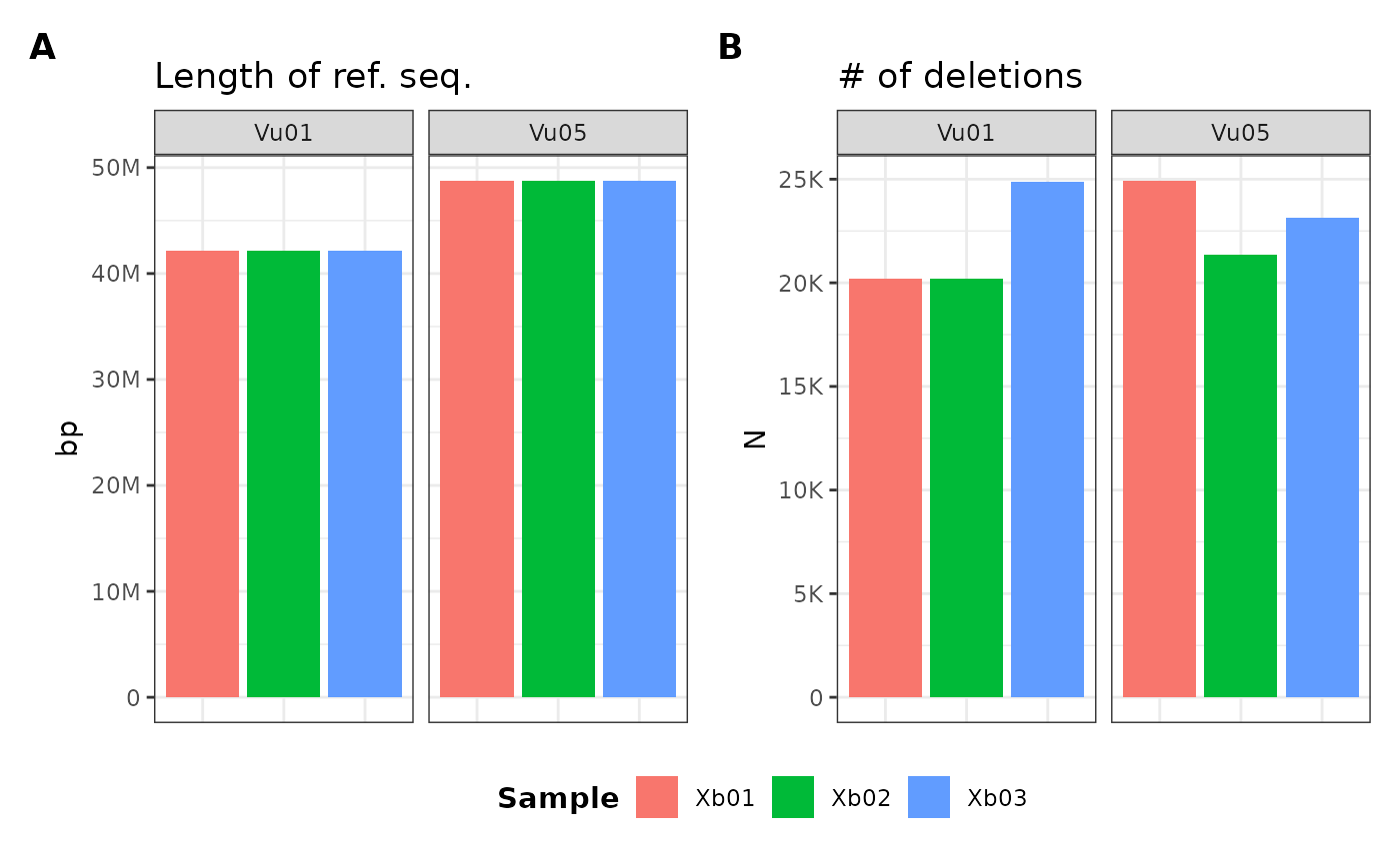

I can also plot the cumulative ALL category which combines all chromosome metrics into one using the ALL keyword on the right-hand-side of the equation:

metData |> plotGvcf(f = ref_length + num_del ~ ALL)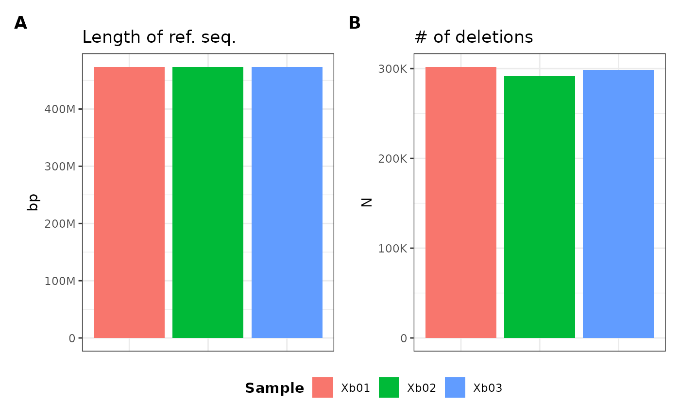

One thing you may have noticed is that the formula parameter is not required. If no formula is used, the default equation will be:

CORE ~ ALL

Dimensions

We can also specify the dimensions of the plot components using two parameters:

number of rows (nRow)
number of columns (nCol)

metData |> plotGvcf(f = ref_length + num_del ~ ALL, nCol = 1)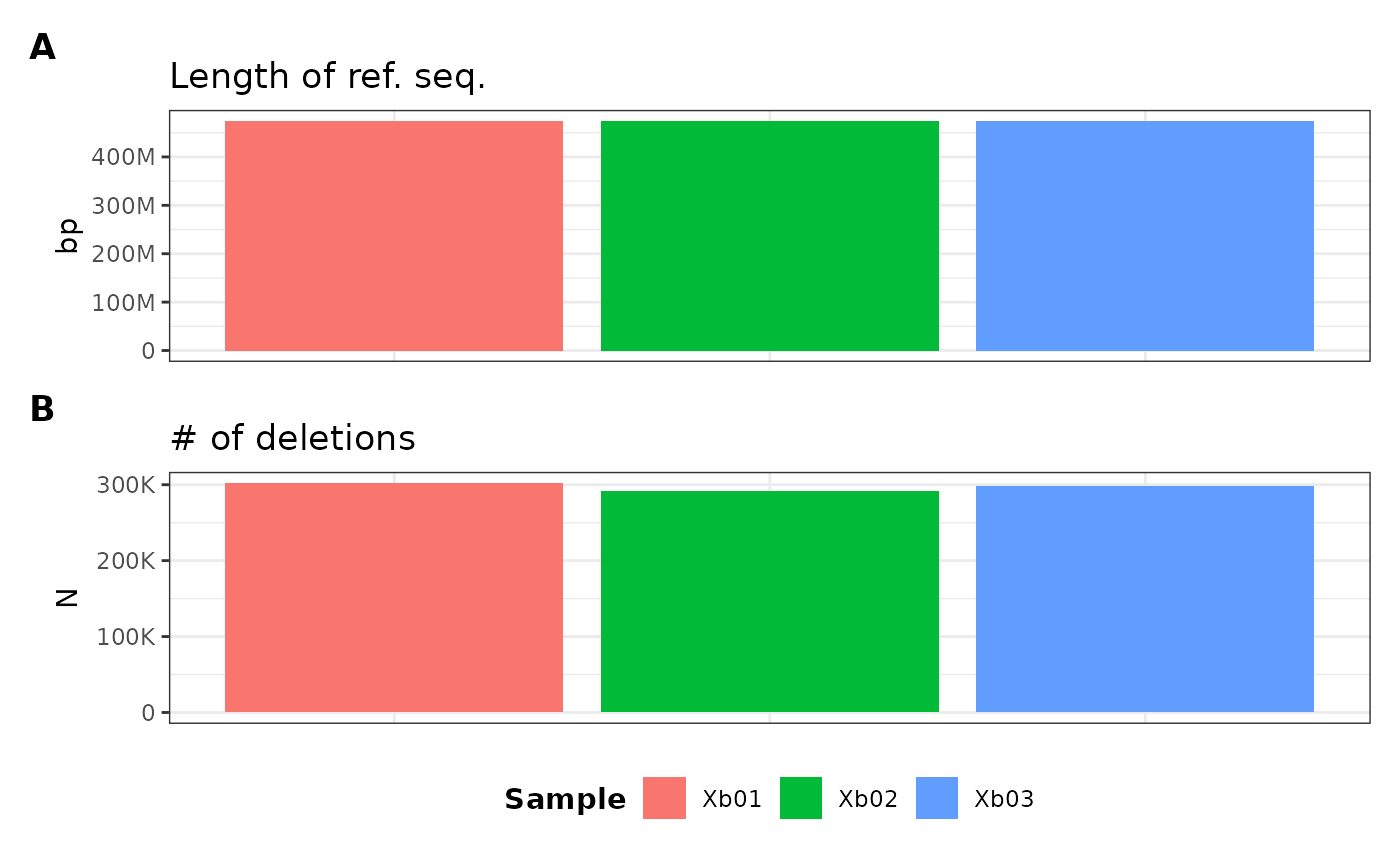

Plot “tags”

We can also modify the tagging type using symbolic identifiers via the tag parameter:

Symbol	Sub plot tag progression
`"A"`	`"A"`, `"B"`, `"C"`, …
`"a"`	`"a"`, `"b"`, `"c"`, …
`"1"`	`"1"`, `"2"`, `"3"`, …
`"I"`	`"I"`, `"II"`, `"III"`, …
`"i"`	`"i"`, `"ii"`, `"iii"`, …

metData |> plotGvcf(f = CORE ~ ALL, tag = "i")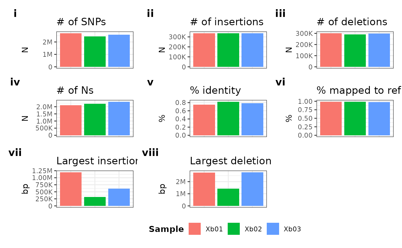

Adding metadata

If you want to color bars based on additional categorical data besides sample ID, you can pass a data.frame object to the parameter mData. This will need the following prerequisites:

A column named either sample, taxa, or line
At least one more column containing a new categorical variable where each sample ID is represented.

In the prior examples, I have 3 samples in my gVCF metrics data:

Xb01
Xb02
Xb03

I will make a data.frame object with following columns: sample, technology, and treatment:

refData <- data.frame(
    sample     = c("Xb01", "Xb02", "Xb03"),
    technology = c("old", "new", "new"),
    treatment  = c("a", "a", "b")
)

refData

##   sample technology treatment
## 1   Xb01        old         a
## 2   Xb02        new         a
## 3   Xb03        new         b

This can now be passed into the mData parameter of plotGvcf():

metData |> plotGvcf(f = CORE ~ ALL, mData = refData)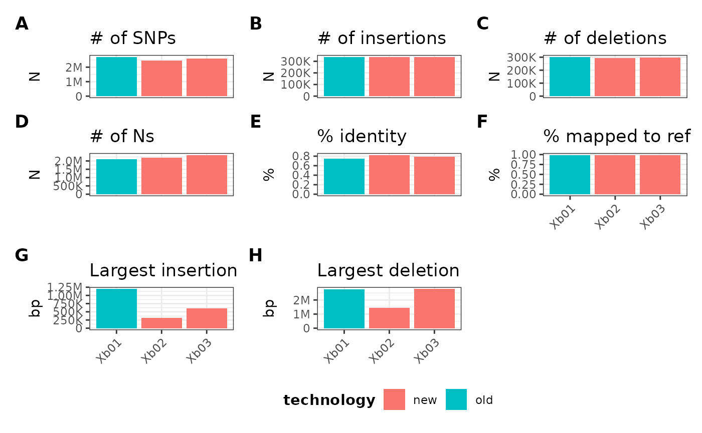

By default, this will pick the first non-sample column in the data.frame object, in this case, technology. We can also specify the column of interest (in case you have multiple columns within your data.frame object) using the mVar parameter:

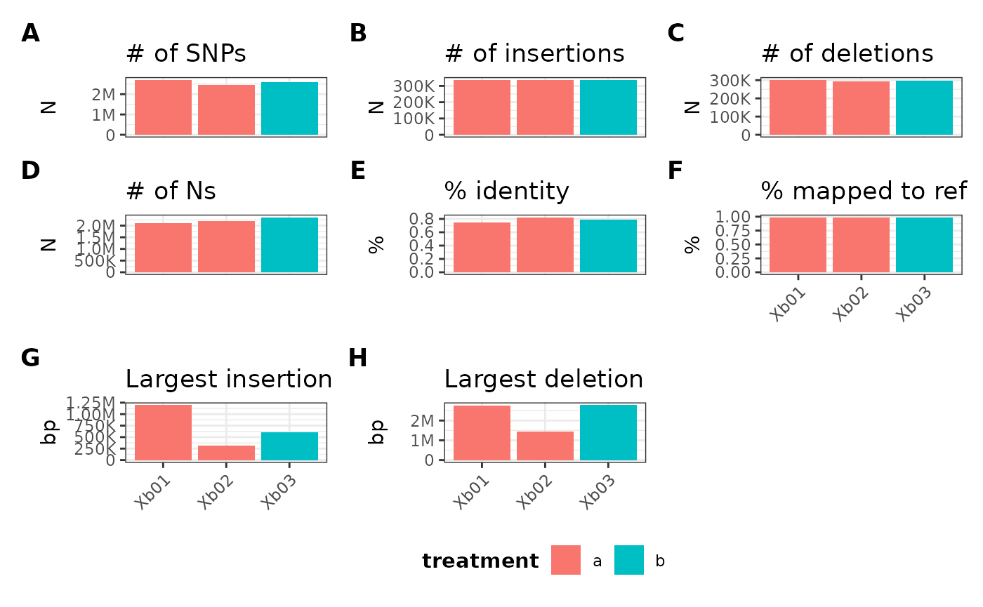
metData |> plotGvcf(
    f = CORE ~ ALL, 
    mData = refData,
    mVar = "treatment"
)

Overriding color

To override default bar coloring (e.g., if you have many samples) to one specified color, you can use the colorOverride parameter:

metData |> plotGvcf(colorOverride = "#73beff")

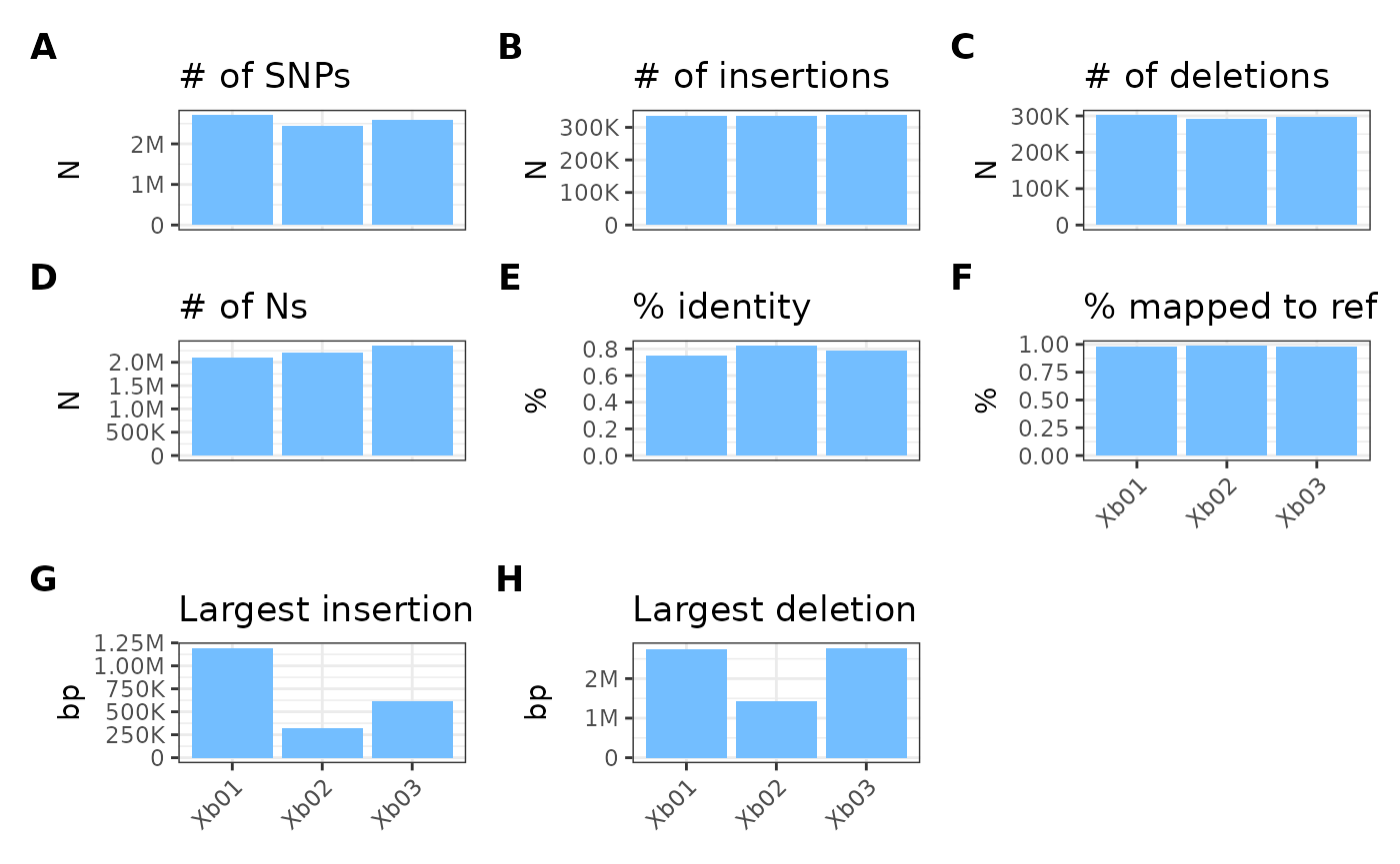
This parameter can also accept R’s default color IDs (i.e., values from the grDevices colors() / colours() function):

metData |> plotGvcf(colorOverride = "forestgreen")

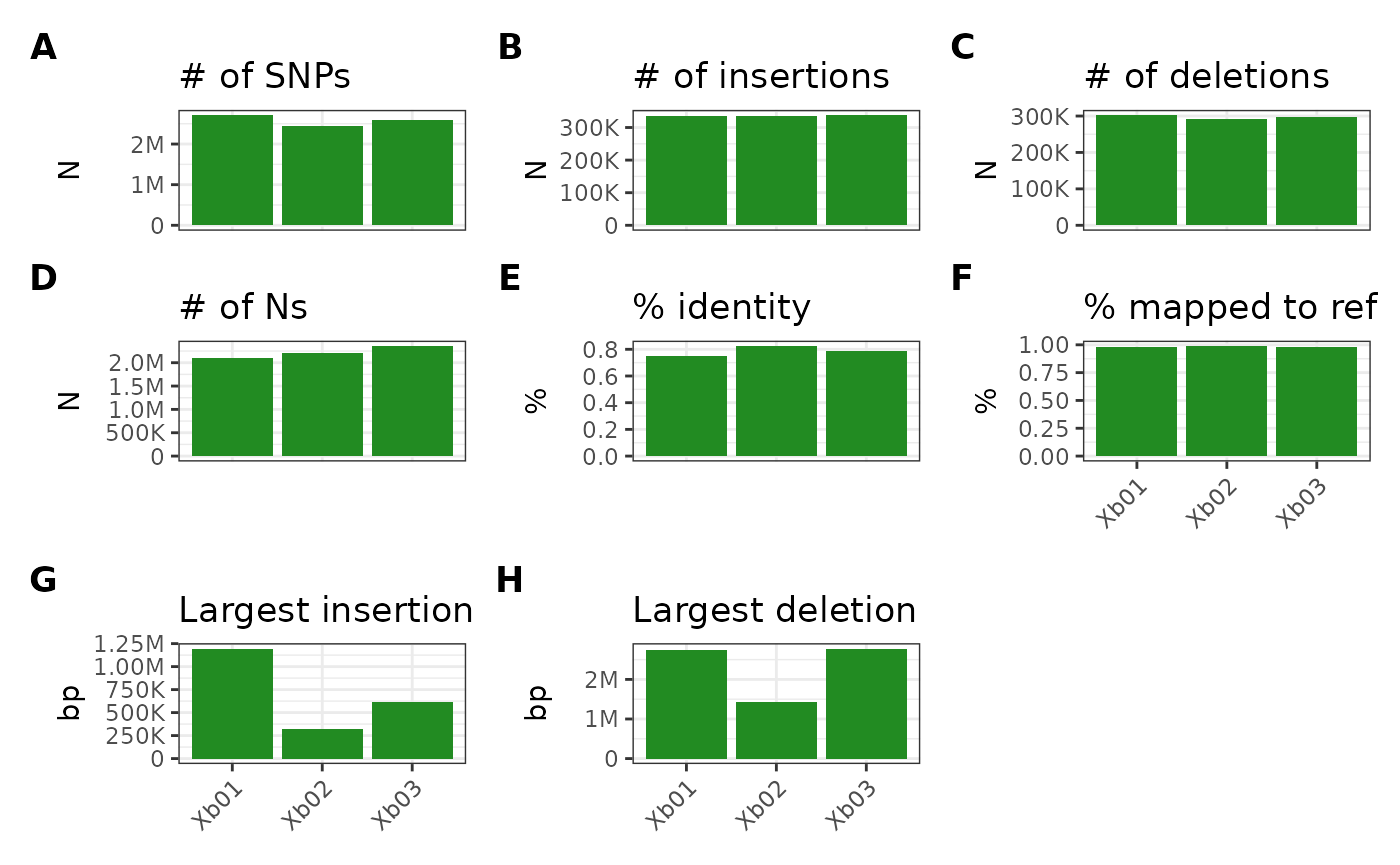
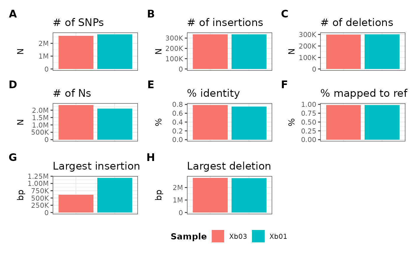
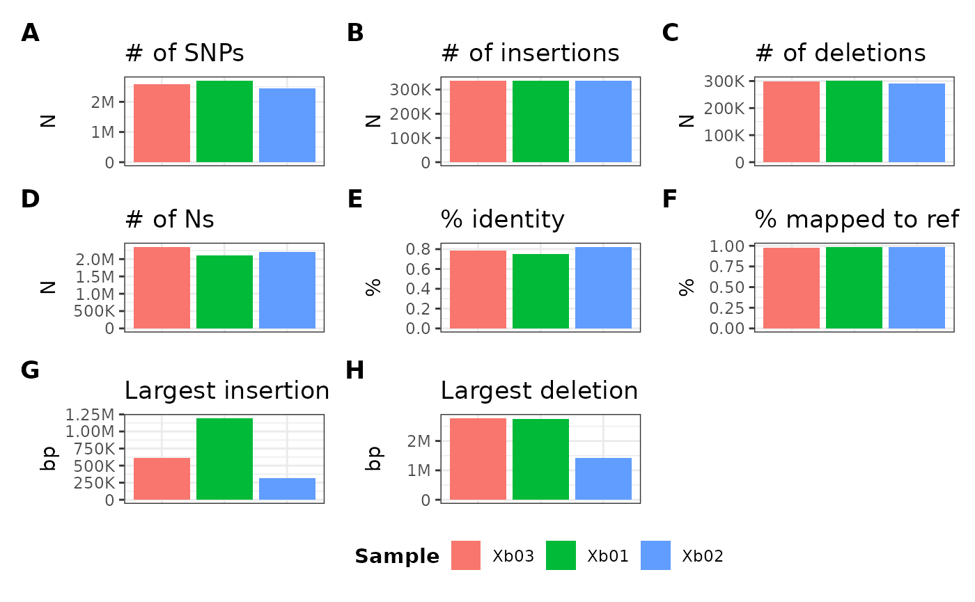
Overriding and filtering sample order

To override the default lexicographic order of sample IDs, you can use the sampleOrder parameter by first defining a character vector of specified order. In the prior examples, the internal sample order is defined as follows:

Xb01, Xb02, Xb03

…if I want to reorder this (e.g., Xb03, Xb01, Xb02), I can use the following example:

newOrder <- c("Xb03", "Xb01", "Xb02")

metData |> plotGvcf(sampleOrder = newOrder)

We can also use this parameter for subsetting samples. For example, If I want to subset the plot to only show values for samples Xb03 and Xb01 and keep them in that order, I can specify the vector as follows:

newOrder <- c("Xb03", "Xb01")

metData |> plotGvcf(sampleOrder = newOrder)

Creating PHGMetrics objects